MAPLE GRAPH FOR COULOMB DAMPED OSCILATION

Together with Mathematica, Matlab, MAPLE is the best choice for computing, programming, and graphing functions.
The syntax of MAPLE is like Pascal.
Javascript, when combined with the appropriate library, for example jsxgraphcore.js can also draw graphs. The syntax of Javascript is like C.
But the syntax of C and Pascal does not differ too much.
Unlike the above tools, the syntax for calculating in Latex is very difficult.
Since programming with MAPLE and Javascript is easier than Latex, I first programmed with Latex, then converted (interpreting) the program to MAPLE and Javascript.

If you have installed Maple 16 but do not know programming with Maple you can learn it by yourself. You can try some following related materials available online:
1- Zhonggang Zeng
An Introduction to Scientific Commputing with Maple Programming (2007)
http://homepages.neiu.edu/~zzeng/340/Fall16/Notes/340book_Old.pdf
2- Bernardin ... Monagan
Maple Programming Guide (2012)
http://www.cybernet.co.jp/maple/documents/pdf/support/documents/Maple16_ProgrammingGuide.pdf
3- Maple 16 User Manual (2012)
https://vdocuments.site/maple16usermanual.html
4- Zhonggang Zeng
Introduction to Scientific Commputing with Maple Programming (2016)
http://homepages.neiu.edu/~zzeng/340/Fall16/Notes/340book.pdf

About the physical aspect of the Coulomb damped oscillation you can read:
1- Singiresu S. Rao
Mechanical Vibrations (page 206: 2.9 Free Vibration with Coulomb Damping)
2- Oscillator damped by a constant-magnitude friction force
https://projects.ncsu.edu/PER/Articles/MarchewkaAbbott&Beichner.pdf

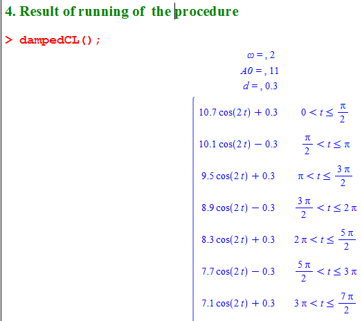
restart;
dampedCL:= proc()
local A0,d,omega,sig,tt,xx,X,n;
omega := readstat("Enter Angular frequency omega = ... rad/s"); 
print(`ω = `, omega);
A0:= readstat("Amplitude (positive or negative number) A0 = ... cm"); 
print(`A0 = `, A0); 
d := readstat("d (2*d is loss of amplitude in half period) d = ... cm"); 
print(`d = `, d); 

n:= ceil((abs(A0)-d)/(2*d));

sig := sign(A0); 
tt := [seq(i*Pi/omega, i = 0 .. n)]; 
xx := [seq((A0-sig*(2*i+1)*d)*cos(omega*t)+sig*(-1)^i*d, i = 0 .. n)]; 
X := piecewise(seq(op([tt[i] < t and t <= tt[i+1], xx[i]]), i = 1 .. n)); 
print(`x(t) = `, X);
with(plots): 
plot(X, t = 0 .. n*Pi/omega);
end;

REMARKS
1. In MAPLE 16, we can export the graph as PDF image:
- Right click the graph.
- Select Export then select Portable Document Format


2. It seems that other than Javascript and Latex, MAPLE is less affected by "Floating point error" (in MAPLE program I do not use function round for (A0 - 2*d*n)).
3. Because the blog does not allow the use of PDF and SVG images, I converted those images into GIF.

NOTE: Sorry! Please fix F_resting to F_restoring

Can also write MAPLE code like Javascript code, for example:





MAPLET coulomb-maplet.mpl

with(plots):with(Maplets[Elements]):
Maplets[Display](Maplet(
Window(title="COULOMB DAMPED OSCILLATION - Enter data then click 'Plot Graph'",resizable=false,
[["omega (rad/s): ",TextField[TF1](value=4),
"Initial displacement a0 (cm): ",TextField[TR1](value=6.2)],
["d = Fcl/k (cm) : ",TextField[TF2](value=0.4),
"Full time of motion (s) : ",TextField[TF4](value="",editable=false)],
["The number of half-periods : ",TextField[TF3](value="",editable=false),
Button[BTN1](caption="Plot Graph", onclick=ACT1)],
Plotter[PL1]()
]), 
Action[ACT1](
Evaluate(TF3='ceil((TR1-TF2)/(2*TF2))'),
Evaluate(TF4='parse(sprintf("%.3f",evalf(round(TF3/TF1*Pi*1000)/1000)))'),
Evaluate(
PL1= 'display(seq((plot((TR1-(2*i-1)*TF2)*cos(TF1*x)+TF2*(-1)^(i-1),x=(i-1)*Pi/TF1..i*Pi/TF1)),i = 1 .. TF3))')
)
));